


Can AI Measure Beauty? A Deep Dive into Meta's Audio Aesthetics Model
A Critical Examination of Meta’s AI Aesthetic Evaluation Model

Can artificial intelligence predict how humans will evaluate the aesthetic qualities of sound? Meta’s researchers believe they’ve developed a framework and model to do exactly that. In their recently released white paper ‘Meta Audiobox Aesthetics: Unified Automatic Quality Assessment for Speech, Music, and Sound¹,’ they propose breaking audio aesthetics into four measurable axes and training models to predict human aesthetic judgments across these dimensions. This analysis will examine both the technical implementation and philosophical implications of their attempt to automate aesthetic evaluation.
This review unfolds in two parts. Part 1 examines the technical foundations: analyzing the model’s construction, evaluating their statistical methodology, and scrutinizing how human annotators were trained to score audio samples. To ground this analysis, I provide detailed examination of three tracks, including my own scoring using their framework. Part 2 offers a theoretical critique, interrogating the assumptions underpinning this project. Building on the flaws uncovered in Part 1, I demonstrate how Meta’s Audiobox Aesthetics model exemplifies how AI’s quantification of human aesthetic experience fundamentally misunderstands and ultimately destroys the very essence it seeks to measure and replicate.
My analysis follows the structure of their paper¹, allowing readers to track Meta’s arguments alongside my critique.
Part 1
In the introduction, the Meta researchers establish the context in which the need for an automated aesthetic predictor is needed. At the root of the issue is the lack of a ‘single ground-truth reference audio in most generative applications.’ A single ground-truth reference is important for evaluating AI-generated audio because, unlike traditional audio processing where you can compare a compressed MP3 to its original uncompressed source, AI-generated audio has no ‘original’ to compare against. This creates a fundamental challenge: how do you evaluate the ‘quality’ of something that has no reference point (hello the entire compendium of theological studies).
This challenge is not unique to music. In image generation, for example, AI models are trained on billions of images and generate new ones through a process that begins with noise. A diffusion model iteratively removes noise in multiple steps, refining the image until it aligns with patterns learned from its training data, the contours of petals, the textures of rock, the way light falls on a cliff. AI-generated music faces a similar issue: without an original source, its ‘quality’ must be inferred from patterns the model has internalized rather than from a direct comparison.
Previous Approaches to Audio Quality Assessment
The development of audio quality assessment has evolved significantly over the last few years across several different domains. In speech analysis, early metrics like PESQ² and POLQA³ set the foundation for evaluating audio quality, but they required an original reference audio file for comparison. This limitation proved problematic for evaluating AI-generated speech, where no ‘original’ exists.
In the broader audio and music domain, the Fréchet Audio Distance (FAD) emerged as a standard metric, calculating the statistical distance between reference and generated audio embeddings from pre-trained models. While FAD showed some correlation with human perception, its statistical nature made it unsuitable for evaluating individual audio samples. This led to the development of neural-based predictors trained on human-annotated quality scores to provide more detailed evaluations. However, these existing methods share several critical limitations. Most focus solely on overall quality scores, which provide little insight into specific aspects of audio that might be problematic.
Meta’s proposed solution attempts to address these limitations through a new annotation guideline with four axes named the aesthetic (AES) scores, which cover several human perceptual dimensions. Their approach aims to cover multiple dimensions of human perception while working across three different types of audio — speech, music, and environmental sounds. They will use the data ‘to train four predictors for non-intrusive and utterance-level automatic audio aesthetic assessment (Audiobox-Aesthetics) models,’ which they have released as an open-source dataset called AES-Natural⁴.
How They Built and Tested Their Model
Having critiqued existing models and methods for evaluating audio quality, the paper proposes four distinct axes through which to capture audio aesthetics. These axes attempt to quantify both technical and subjective aspects of audio quality:
1. Production Quality (PQ) Focuses on the technical aspects of quality instead of subjective quality. Aspects including clarity & fidelity, dynamics, frequencies and spatialization of the audio;
2. Production Complexity (PC) Focuses on the complexity of an audio scene, measured by number of audio components;
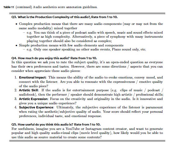
3. Content Enjoyment (CE) Focuses on the subject quality of an audio piece. It’s a more open-ended axis, some aspects might includes emotional impact, artistic skill, artistic expression, as well as subjective experience, etc;
4. Content Usefulness (CU) Also a subjective axis, evaluating the likelihood of leveraging the audio as source material for content creation
These four categories represent Meta’s attempt to quantify those ineffable qualities that audio and music embody, providing the framework through which their human annotators will score audio samples.
Now before we get into the fun part of this paper which involves how they hired and trained human annotators to create their ‘ground-truth’ dataset, I want to highlight my qualifications that I see are relevant to this analysis.
I spent 17 years as a music analyst for Pandora Radio’s Music Genome Project⁵, where I worked with a team of highly trained analysts who meticulously evaluated over 400 variables per song, including non-musical audio such as comedy. This analytical experience was built upon my career as a session musician where I recorded on hundreds of records and as a touring musician, traveling globally with dozens of artists after receiving my degree in Studio Music and Jazz Drum Set Performance from the University of Miami in the 90's.
Beyond music, my analytical approach is shaped by graduate work in Public Policy and Administration, where I developed expertise in statistical analysis and research methodology, including experience as a graduate research assistant. Combined with my long-standing engagement with philosophy and aesthetics, this diverse yet domain-specific background allows me to critically evaluate both Meta’s dataset methodology and its implementation in model training.
With these qualifications established, let’s examine how Meta approached the audio sample collection and the human evaluation of their audio samples across their three categories: speech, sound effects, and music.
The Audio samples were drawn from open-source and licensed datasets across the three modalities mentioned before — speech, sound effects, and music. They performed stratified sampling using available metadata (speaker ID, genre labels, demographics) where it existed, though the paper doesn’t specify how comprehensive this metadata was or what gaps might exist. All audio was normalized for loudness to prevent volume differences from skewing ratings, and each sample received three independent ratings to reduce variance (the choice of three rather than two or five or ten is significant as well).
Meta’s team first sought to create a ‘golden set’ of audio samples scored by experts, which then served as the ‘ground-truth.’ Potential raters (i.e. people interviewing for the job) were evaluated against this master set, with particular attention paid to their ability to assess production quality (PQ) and production complexity (PC). These were chosen because they are more ‘technically objective’ measures. Only individuals achieving a Pearson correlation greater than 0.7 with the expert ratings were selected. This process yielded 158 raters who, according to the researchers, represented a ‘diverse subjective opinions from the general public.’
The instructions provided to their human annotators in Appendix B reveal an interesting set of decisions which will have profound consequences for their model which I will address throughout.

The team of 158 raters (in the paper they switch between annotators and raters and I am going to do the same) then analyzed approximately 500 hours of audio, comprising 97,000 samples evenly distributed across speech, sound, and music. Each sample was between 10–30 seconds in length. While this might seem like a substantial dataset, it’s worth noting that in my work at Pandora, I personally analyzed nearly 18 times more than their entire dataset across all three modalities combined.
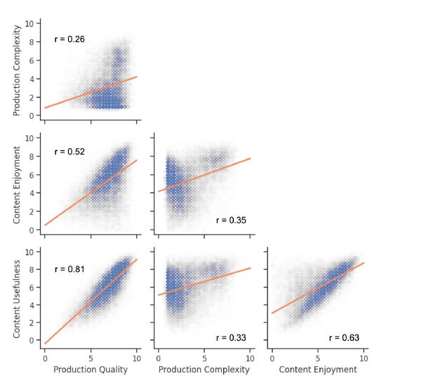
Their correlation analysis (Figure 2) reveals several interesting patterns. The strongest correlation (r = 0.81) appears between Production Quality and Content Usefulness, suggesting that better-produced audio is generally rated as more useful (useful for whom and what?). However, Production Complexity shows surprisingly weak correlations with other measures (r = 0.26 with Production Quality, r = 0.35 with Content Enjoyment). The researchers interpret these weak correlations as justification for treating these measures independently, but this interpretation is problematic.
Critique 1
First, they’ve combined all three modalities (speech, sound, and music) into a single correlation matrix, despite acknowledging that these modalities have different characteristics — they note that ‘music in general has higher production complexity than speech and sound effects.’ This aggregation obviously masks important differences in how these measures relate within each modality. A more rigorous approach would have been to show separate correlation matrices for speech, sound, and music. I am baffled why they combined sound effects with music production and plain speech together.
This would explain the variance in production quality and production complexity correlation, as their human raters are rating speech as low in production complexity compared to a fully produced piece of music. However, in the real world, an embodied human being will associate a speech recorded, for example, from an audiobook as high in complexity than versus a recording of someone speaking through a phone’s speaker. This crucial distinction, which I consider substantial, is lost in their analysis by combining speech, sound effects, and music within a single correlation matrix.
This problem could have been addressed differently through changing the construction of Question 3 in the rater training handout they produced (Appendix B)¹. The raters could have been instructed that even though speech might seem simpler in production compared to a fully produced song, they should judge each modality within its own context — evaluating audiobook production quality against other audiobooks or against a recording of someone speaking from a smartphone speaker, for instance, rather than against a fully produced and orchestrated song as they instruct in Question 3. From my vantage point as someone who has both produced professional audio and trained other analysts during my time at Pandora, this is an amateur mistake that suggests a fundamental lack of real-world audio expertise on the research team.
Second, I have significant concerns with the fact all audio was normalized for loudness to prevent volume differences from skewing ratings. This normalization process is problematic because of what normalization does to the audio. It takes the lowest dynamic level (volume) and raises it while lowering (compressing) the highest dynamic level so that the overall loudness is uniform compared to other audio samples being used or a standardized loudness level. Which normalizing method they use is not disclosed (LUFS, Peak, RMS) and that too matters for the severity of the normalizing effect on the audio sample.
As a professional musician, I can tell you unequivocally that dynamic range is the most important aspect of expression and is at the core of any aesthetic style within a musical performance. Normalization flattens the very aesthetic human expressive function they are purportedly attempting to capture.
Now you may say, ‘But we are dealing with speech and sound effects, not just music.’ Oh please, humans react just as much to dynamics in any audio context. Think of how a whispered threat carries more weight than a shouted one, or how the sudden silence after the end of a shout or clap of thunder enhances its impact. The aesthetic meaning of any sound, whether speech, music, or environmental noise, emerges from its dynamic relationship to its context. This decision to normalize the audio at this stage will transmit throughout the chain of the model training that will transpire.
Thirdly, I would caution against using metadata as a basis for analyzing audio. Metadata is often inaccurate and embeds cultural signifiers that, rather than providing an objective music viz music framework, reinforce subjective cultural symbols — the very biases this model claims to transcend. The paper does not specify exactly how metadata is incorporated into the model or what weighting is applied to this data, making it impossible to determine whether this is a significant flaw or a minor quibble.
Fourthly, the dataset itself is strikingly small. 500 hours of annotated audio, spread across speech, sound, and music, is practically negligible. As I noted earlier, my personal contribution to the Music Genome Project alone amounted to many times this volume, and while that work spanned years, it was also conducted by a sizable team. At best, this dataset is a starting point, but it is far from comprehensive enough to produce outputs that can be reliably acted upon.
Fithly, assessing the error correlation between different members of the analysis team is difficult without conducting my own evaluation of what constitutes a meaningful match between one person’s analysis of a sound sample and another’s. Is r = 0.7 a strong enough correlation to ensure reliable annotations for model training? The paper does not provide enough context to make that determination. An r = 0.7 suggests a moderate to strong correlation, meaning that while raters generally align in their scoring, there is still a notable degree of variance. However, without knowing the actual distribution of scores or how frequently raters significantly diverged, it’s impossible to determine whether this threshold was chosen arbitrarily or represents a genuinely rigorous standard.
Having three raters score the same audio sample is a significant methodological choice, as it directly impacts dataset coherence. But what happens when the three raters disagree? If their Pearson correlation is low — say, 0.3 or 0.6 — what does the Meta team do with that data? Are they averaging the three scores into a single value regardless of disagreement, or are they applying a quality control filter that flags samples with low agreement for additional review before they are used in training?
The latter approach would be far more effective for maintaining dataset consistency over time. While I agree that three raters per sample is a reasonable number (as opposed to five or ten), how those three ratings are processed is crucial. If outliers are not accounted for, the dataset could end up encoding noise rather than refining a predictive framework.
Sixthly, since we are dealing with aesthetic scoring, what are these individuals personal backgrounds? Did they go to college? Are they computer scientist or pianters, musicians, chefs, athletes, mothers, fathers, CEO’s, day laborers, mechanics, day traders etc etc. I mean we are focusing on aesthetics here right? I’ll explore this more in Part 2.
The Math
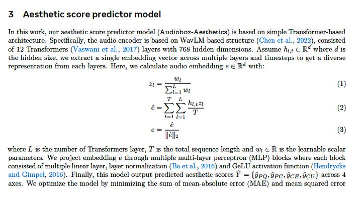
The core of Meta’s approach is the Audiobox-Aesthetics (AES) model, which utilizes a transformer-based architecture similar in structure to those used in large language models. However, instead of processing text, this model is designed to analyze audio by extracting structured representations from raw waveforms. The model processes audio through a series of steps:
WavLM Encoder: The model first converts raw audio into numerical representations (embeddings) using WavLM⁶, a self-supervised speech representation model. This step transforms the waveform into structured data the transformer can process.
Transformer Layers: These embeddings then pass through 12 Transformer layers, which extract patterns and hierarchical features across different time scales in the audio.
Multi-Layer Representation: The model aggregates information across the layers to form a richer representation of the input audio.
Finally, it uses this representation to predict scores for each of the four aesthetic measures (Ŷ = {ŷPQ, ŷPC, ŷCE, ŷCU} — Production Quality (PQ), Production Complexity (PC), Content Enjoyment (CE), and Content Usefulness (CU)).
The mathematical equations shown perform these functions:
zₗ = wₗ/∑ᴸₗ₌₁wₗ — This equation represents the weight assigned to each layer in the final representation.
ê = ∑ᵀₜ₌₁∑ᴸₗ₌₁ hₗ,ₜzₗ/T — Here, the model combines feature representations from all layers and across time, normalizing them with the assigned weights.
e = ê/||ê||₂ — This ensures that the final representation has unit length, preventing any one feature from dominating due to scale differences. This is a form of normalization in the statistical sense (not in the music loudness sense).
While the mathematics looks complex, the essential idea is straightforward: the model learns to transform raw audio waveforms into numerical scores that attempt to capture different aspects of audio quality through this process.

The Architecture Diagram illustrates how their model processes audio:
Input: Audio waveform at 16 kHz.
Feature Extraction: CNN Encoders process the raw waveform, extracting low-level acoustic features for further analysis.
Temporal Understanding: A Transformer Encoder further processes these features, capturing long-range dependencies and structural relationships in the audio.
Final Predictions: Four separate Multi-Layer Perceptrons (MLPs) each predict one aesthetic score (scores from from Figure 3 above):
Production Quality (PQ): predicts 8.0
Production Complexity (PC): predicts 5.6
Content Enjoyment (CE): predicts 7.5
Content Usefulness (CU): predicts 3.2
The Loss Function: L = Σ (ya — ŷa)² + |ya — ŷa| where a ∈ {PQ, PC, CE, CU}
This equation shows how they measure error for each aesthetic measure (PQ, PC, CE, CU):
ya is the actual human rating (ground-truth)
ŷa is the model’s prediction
Two types of error are calculated:
Squared Error (ya — ŷa)²: Penalizes larger errors more heavily, making the model more sensitive to big mistakes.
Absolute Error |ya — ŷa|: Applies a linear penalty, preventing extreme corrections and helping with stability.
let’s walk through a concrete example:
Input: A piece of audio gets processed through their system as 16kHz
Output: The model predicts four scores
These predictions are compared against human ratings
Let’s say for one aesthetic measure:
Human rater gave it a 7 (ya)
Model predicted a 4 (ŷa)
Then:
Squared error: (7–4)² = 9
This punishes bigger mistakes more because squaring makes big numbers much bigger
If the model was off by 6 points instead of 3, the squared error would be (7–1)² = 36, amplifying the penalty for larger mistakes.
Absolute error: |7–4| = 3
This is just the straight difference
Keeps the error in the same scale as the original ratings
They add both types of errors together because:
Squared error helps the model avoid big mistakes
Absolute error helps keep the predictions generally close to human ratings
So for this example: L = (7–4)² + |7–4| = 9 + 3 = 12
They do this for each of their four aesthetic measures (PQ, PC, CE, CU) and sum it all up to get their total loss that they try to minimize during training. The final loss function sums the individual errors across all four aesthetic dimensions.
The Algorithm
Algorithm 1 Audio Aesthetic Inference
Require: x: audio input, sr: sample rate
Ensure: y_pred: predicted aesthetic score
1: Initialize lens ← [], preds ← []
2: stepsize ← sr × 10
3: for t ← 0 to len(x) with step stepsize do
4:    xnow ← x[t × stepsize : (t + 1) × stepsize]
5:    Append AES(xnow) to preds
6:    Append len(xnow) to lens
7: end for
8: w ← lens/sum(lens)
9: y_pred ← sum(preds × w)
10: return y_pred
This is their Audio Aesthetic Inference algorithm. It follows a straightforward structure, but some of its design choices, especially its method of processing audio in discrete chunks, warrant closer examination later on.
First it ingests the audio. we know the sample rate will be 16 Hrz.
It creates two columns a lens column and a prediction column, and then it splices the audio into 10 second chunks. A 32-second piece of audio would look like this:
# After first 10-second chunk:
preds = [score_for_chunk_1]
lens = [10]

# After second chunk:
preds = [score_for_chunk_1, score_for_chunk_2]
lens = [10, 10]

# After third chunk:
preds = [score_for_chunk_1, score_for_chunk_2, score_for_chunk_3]
lens = [10, 10, 10]

# After final 2-second chunk:
preds = [score_for_chunk_1, score_for_chunk_2, score_for_chunk_3, score_for_chunk_4]
lens = [10, 10, 10, 2]
Steps 3, 4, 5, and 6 are where the core processing of the algorithm happens. Each 10-second chunk and the final 2-second chunk is extracted from the original audio and passed into their Audiobox-Aesthetics model (AES).
In Step 5, each xnow segment is processed by the AES model, which outputs a set of those four aesthetic scores: Production Quality (PQ), Production Complexity (PC), Content Enjoyment (CE), and Content Usefulness (CU).
These scores are stored in preds, which keeps track of all the chunk-level aesthetic ratings. Simultaneously, Step 6 logs the length of each chunk in lens, which later helps in weighted averaging to ensure longer chunks influence the final prediction proportionally.
The weighted averaging using some random scores I chose works thusly:
# Calculate weights for each chunk
w = lens/sum(lens)
# For our 32-second example:
lens = [10, 10, 10, 2]
sum(lens) = 32
w = [0.3125, 0.3125, 0.3125, 0.0625]
# PQ final score
y_pred_PQ = sum([7.5*0.3125, 8.0*0.3125, 7.0*0.3125, 6.5*0.0625])

# PC final score
y_pred_PC = sum([6.8*0.3125, 7.2*0.3125, 7.5*0.3125, 7.0*0.0625])

# CE final score
y_pred_CE = sum([8.2*0.3125, 8.0*0.3125, 7.8*0.3125, 7.5*0.0625])

# CU final score
y_pred_CU = sum([7.0*0.3125, 6.5*0.3125, 6.8*0.3125, 6.0*0.0625])
In this example (with made-up predicted scores), we obtain a final weighted score for each of the four aesthetic dimensions:
y_pred_PQ = 7.4375 (Final Production Quality Score)
y_pred_PC = 7.15625 (Final Production Complexity Score)
y_pred_CE = 7.96875 (Final Content Enjoyment Score)
y_pred_CU = 6.71875 (Final Content Usefulness Score)
Critique 2
I want to focus on these 10-second chunks. I have taken the time to break down the math and algorithm, not just for its technical details, but to expose the aesthetic choices embedded in the model’s design. These are choices made by engineers that shape how the model “hears” and evaluates sound.
From the outset, the model is framed as an objective system. It emphasizes the recruitment of trained human listeners to establish a ground-truth golden dataset. This methodology is presented as purposive, empirical, and neutral. It forms the foundation upon which the AES model is trained.
But what is being elided in this framing is the subjective, arbitrary, and aesthetic nature of the model’s own design.
Think of a song. A standard pop song lasts between three and four minutes. Would you say your emotional relationship to that song can be quantified into 10-second slices? When you listen to a song, are you only listening to the immediate sonic and technical aspects, or are you already envisioning and embodying a gestalt, a coherent whole through which your relationship with the unfolding song manifests?
Yes, the model is designed to take each 10-second slice, normalize it, and sum its predictions to produce an overall score for the song. But think about the violence in this process. The flattening of dynamics. The atomization of a heterogeneous, temporal, expressive medium. The arbitrariness of where that 10-second cut happens. Does it occur three seconds before the four-second tag of the second verse which is just before the 27-second chorus, which is orchestrated with completely different instruments? And how does the model account for that four-second tag — appearing only once in the entire song — yet carrying a sense of longing that no other moment expresses?
It doesn’t. It can’t. The model is designed to flatten those aesthetic aspects into nullity.
Alright, let’s look at the model results. I am going to skip the section that focuses on speech and sound effects and focus solely on the music samples for the sake of length.

The AES Model Results
# Table 2: Utterance-level Pearson Correlation Coefficient between two types
   #  of human annotations: AES and OVL on PAM sound and music test sets.

              +-------------+-------+-------+-------+-------+
              | Test set    | GT-PQ | GT-PC | GT-CE | GT-CU |
              +-------------+-------+-------+-------+-------+
              | PAM-sound   | 0.496 | 0.190 | 0.581 | 0.486 |
              | PAM-music   | 0.778 | 0.490 | 0.848 | 0.804 |
              +-------------+-------+-------+-------+-------+
# Table 4: Utterance-level Pearson Correlation Coefficient between
# human-annotated and predicted scores on PAM-music.
| Model | OVL | GT-PQ | GT-PC | GT-CE | GT-CU |
|---------------------------|------|-------|-------|-------|-------|
| PAM | 0.581| 0.568 | 0.377 | 0.699 | 0.573 |
|---------------------------|------|-------|-------|-------|-------|
| Audiobox-Aesthetics-PQ | 0.464| 0.587 | 0.193 | 0.449 | 0.537 |
| Audiobox-Aesthetics-PC | 0.251| 0.113 | 0.710 | 0.322 | 0.096 |
| Audiobox-Aesthetics-CE | 0.528| 0.487 | 0.455 | 0.615 | 0.488 |
| Audiobox-Aesthetics-CU | 0.465| 0.594 | 0.221 | 0.502 | 0.558 |The Meta team used a baseline model to test their AES model against: the PAM model⁷.
The PAM model is an existing framework for evaluating audio quality. It was developed as part of a study by Deshmukh et al. and is used in this white paper as a benchmark for comparing the performance of Meta’s AES model.
PAM includes a dataset of 500 music samples, known as PAM-music, which consists of 100 natural recordings and 400 AI-generated pieces from various generative models (audioldm2, musicgen_large, musicgen_melody, musicldm). Each sample was annotated by 10 human raters, who assigned an Overall Quality (OVL) score based on their perception of the music, which is averaged into one OVL score. In addition each music clip has a descriptive narrative, for example:
You can hear birds chirping along with pig-sounds. Then a full orchestra with strings bell sounds and a choir comes rising in tension. This song may be playing in a dramatic epic movie scene. — clip title: YwUa3OS92ZQ⁷
From my review of the dataset, I observed that the original audio files are typically 10s, mono, and 22 kHz, while AI-generated samples tend to be 5s and 16 kHz
The purpose of the PAM model is to predict how humans would rate the overall quality of a given piece of music. It is designed to capture general perception rather than discrete aesthetic categories. Meta, however, uses PAM as a benchmark to assess how well their Audiobox-Aesthetics model aligns with human judgment.
I want to stress what is happening here because it is not obvious in the two tables above. A pre-existing dataset, PAM-music, hired 10 human raters to give one overall quality score (PAM-OVL) on a 1–5 scale for entire tracks. Meta then hired and trained an additional 10 human raters with audio-related backgrounds to re-evaluate these same tracks using the four newly defined aesthetic axes — Production Quality (GT-PQ), Production Complexity (GT-PC), Content Enjoyment (GT-CE), and Content Usefulness (GT-CU) — each rated on a 1–10 scale. Meta then tested how well their AES model’s predictions correlated with these newly assigned GT scores and also examined how well the four GT scores aligned with the original PAM-OVL ratings across both the 100 original tracks and 400 AI-generated tracks.
Table 2 shows the correlation between sound (non-music) and music. As I mentioned earlier I am only focused on the music. We can see there is a strong correlation for three of the AES axis, with Production Quality being the weaker correlation.
Table 3 is a full correlation matrix which shows that the PAM model has a stronger correlation with human-assigned OVL ratings than the Audiobox-Aesthetics model. This suggests that PAM is better at capturing the holistic experience of music, while Meta’s model, struggles to generalize to overall perception. The ground truth (GT) annotations that Meta created are tightly correlated to their corresponding AES predictor, but when you look at the other correlations, they are weak, with some so low that they are effectively meaningless outside their training label (GT-PQ to Audiobox-PC (0.113), GT-CU to Audiobox-PC (0.096)). This confirms that the AES model is overfitted to its own aesthetic framework and fails to generalize beyond the dataset it was specifically trained on.
Meta attributes the slightly worse performance of their AES predictors (compared to PAM) in music to the fact that they did not use synthetic (AI-generated) data in training:
The slightly worse performance of the proposed AES predictors compared to PAM, especially in music, might be caused by the unseen data issue that we did not use any synthetic data to train the Audiobox-Aesthetics models.
I disagree with this assessment.
The AES-Natural Dataset and Meta’s Internal Benchmarking
After testing their Audiobox-Aesthetics model against the PAM-music dataset, the Meta team shifts to evaluating it on their own in-house dataset, AES-Natural. Unlike PAM, which was an independent benchmark, AES-Natural was constructed from publicly available datasets such as MUSDB18-HQ⁸, MusicCaps⁹, and AudioSet¹⁰ for the music sources. Meta curated a subset of 1,000 music samples, each ranging from 20 to 50 seconds, to serve as the new testing ground for their model.
Unlike PAM, which relied on a single overall quality (OVL) rating, AES-Natural was annotated from scratch using Meta’s four aesthetic axes (PQ, PC, CE, CU) by a team of 10 in house raters (most likely the same as the team who scored the PAM samples but this is not explicitly stated). This means that rather than testing their model against an external standard, they are now testing it on a dataset built to align with their model’s assumptions.
To further evaluate performance, they compare PAM and Audiobox-Aesthetics predictors on this new dataset. This table below presents the Pearson Correlation Coefficients between the 10 person human-annotated ground-truth scores and the predicted scores from each system.
# Table 7: Utterance-level Pearson Correlation Coefficient between
# human-annotated and predicted scores on AES-Natural (Music)

| Model                     | GT-PQ  | GT-PC  | GT-CE  | GT-CU  |
|---------------------------|--------|--------|--------|--------|
| PAM                       | 0.402  | -0.293 | 0.250  | 0.284  |
|---------------------------|--------|--------|--------|--------|
| Audiobox-Aesthetics-PQ    | 0.888  | -0.538 | 0.783  | 0.834  |
| Audiobox-Aesthetics-PC    | -0.538 | 0.700* | 0.604  | -0.677 |
| Audiobox-Aesthetics-CE    | 0.783  | -0.544 | 0.859  | 0.886  |
| Audiobox-Aesthetics-CU    | 0.834  | -0.565 | 0.835  | 0.876  |
We can see that when the PAM model is tested against the AES-Natural music dataset, it does not perform well — at all. This alone should raise questions about whether AES-Natural reflects an independent measure of musical quality or whether it is an engineered benchmark designed to validate Meta’s framework.
They claim:
According to the results of Table 5–7, we find that the production complexity is decoupled from the other three AES axes, and the Audiobox-Aesthetics-PC achieves a high prediction accuracy, so the proposed PC predictor provides an irreplaceable novel view for audio quality evaluations.
So let’s look at some of these claims and the actual scoring of the four AES axis.
Critique 3
In Critique 1, I pointed out how Meta is combining music, speech, and sound effects into a single framework despite acknowledging their vastly different characteristics. Table 7 further confirms the issue: Production Complexity (PC) shows negative correlations with Production Quality (PQ), Content Enjoyment (CE), and Content Usefulness (CU).
This pattern is not limited to the music dataset but holds across all three auditory modalities — speech, sound, and music. Looking at Tables 5 and 6, which show utterance-level Pearson Correlation Coefficients between human-annotated and predicted scores, we see that Production Complexity (PC) is an outlier in every case. I have marked this with an asterisk (*) for clarity:
# Table 5: Utterance-level Pearson Correlation Coefficient between
# human-annotated and predicted scores on natural speech

| Model                     | GT-PQ  | GT-PC  | GT-CE  | GT-CU  |
|---------------------------|--------|--------|--------|--------|
| PAM                       | 0.317  | -0.292 | 0.250  | 0.284  |
| DNSMOS                    | 0.662  | -0.462 | 0.589  | 0.632  |
| SQUIM                     | 0.660  | -0.466 | 0.570  | 0.604  |
| UTMOSv2                   | 0.603  | -0.358 | 0.574  | 0.588  |
|---------------------------|--------|--------|--------|--------|
| Audiobox-Aesthetics-PQ    | 0.888  | -0.538 | 0.783  | 0.834  |
| Audiobox-Aesthetics-PC    | -0.693 |  0.700*| -0.643 | -0.677 |
| Audiobox-Aesthetics-CE    | 0.879  | -0.544 | 0.859  | 0.886  |
| Audiobox-Aesthetics-CU    | 0.898  | -0.565 | 0.835  | 0.876  |
# Table 6: Utterance-level Pearson Correlation Coefficient between
# human-annotated and predicted scores on natural sound
| Model | GT-PQ | GT-PC | GT-CE | GT-CU |
|---------------------------|--------|--------|--------|--------|
| PAM | 0.462 | -0.022 | 0.438 | 0.443 |
|---------------------------|--------|--------|--------|--------|
| Audiobox-Aesthetics-PQ | 0.728 | -0.014 | 0.552 | 0.655 |
| Audiobox-Aesthetics-PC | 0.106 | 0.758*| 0.297 | 0.017 |
| Audiobox-Aesthetics-CE | 0.492 | 0.288 | 0.763 | 0.466 |
| Audiobox-Aesthetics-CU | 0.676 | 0.012 | 0.571 | 0.644 |Meta’s Production Complexity metric lacks a coherent definition across different audio types, as evidenced by its erratic correlation patterns across Tables 5, 6, and 7. If the same metric produces drastically different correlations across speech, sound, and music, it suggests that raters are being forced to evaluate complexity through an artificially imposed, context-independent rubric. Appendix B shows how Meta defines complexity to the raters they hired:

As I argued earlier, an audiobook recorded in a professional studio compared to a voice of someone speaking out of a smartphone speaker, is more than just quality there is a complexity that needs to be understood in context. When this is grouped with a fully produced song, these distinctions are flattened because raters are forced to apply a single framework across all audio types.
This definition of complexity is deeply flawed. By treating the mere presence of multiple audio elements as inherently complex, Meta ignores actual musical or production intricacy. A symphony with melodies and harmonies weaving across instruments and sections, is not equivalent to a podcast with layered background music, yet both are labeled ‘complex’ under this framework. A pianist using complex modal harmony as opposed to a piano playing root position triads is vastly different in complexity across, technique, style, temporal symbolic forms, and aesthetic historicity.
But, I can hear Meta’s team screaming at me, (maybe rightfully so) Production Quality is where we capture this! OK let’s review this:

When I read these instructions I imagine this would result in a strong negative correlation between Production Quality (PQ) and Production Complexity (PC) when analyzing speech, and a more flexible but still negative relationship in music. In other words, a professionally recorded audiobook should exhibit high PQ and low PC, while a voice captured through a smartphone speaker should have both low PQ and low PC. For music, the correlation should be more nuanced. Let's consider a lo-fi, super-compressed, narrow-spatialized recording of a banjo player accompanying a symphony orchestra at an outdoor bluegrass festival, captured with a Tascam handheld field recorder. According to Meta’s framework, this should be high PC (due to the number of sonic elements) but low PQ (due to recording artifacts and lack of fidelity).
Looking at the data from the white paper, Table 5 (natural speech) confirms a strong negative correlation between PQ and PC (-0.538 in Audiobox-Aesthetics, -0.292 in PAM). This aligns with expectations that the more ‘complex’ a speech recording is judged to be, the lower its production quality score. However, in Table 6 (natural sound), this relationship weakens (-0.014 in Audiobox-Aesthetics, -0.022 in PAM), suggesting that complexity and quality are less tightly coupled for non-music, non-speech sounds which I would attribute to a possible category error in scoring ‘natural sounds’ within this framework. In Table 7 (music), PQ and PC maintain a strong negative correlation (-0.538 in Audiobox-Aesthetics, -0.293 in PAM), which aligns with the framework’s assumptions: a track can be highly produced and sonically refined (high PQ) while remaining relatively simple in its arrangement or instrumentation (low PC). For instance, a solo jazz guitar recording, despite being meticulously recorded and mixed, might only register a 1 or 2 on the PC scale due to its lack of layered elements.
This raises deeper concerns about how complexity is being defined across different audio domains. If a symphony with carefully interwoven harmonies and counterpoint is treated as ‘complex’ in the same way as a podcast with layered background music, then the metric is conflating structural complexity (musical intricacy) with surface-level complexity (the presence of multiple audio elements). This distinction is crucial, as failing to account for the qualitative nature of complexity risks misleading correlations.
Table 5 supports this concern: Audiobox-Aesthetics-PC scores 0.700 for Production Complexity, but has strong negative correlations with Content Enjoyment (-0.643) and Content Usefulness (-0.677). This suggests that, under Meta’s framework, more “complex” speech recordings tend to be rated as less enjoyable and useful. One plausible explanation is that the metric is capturing cases where speech is overlaid with excessive background elements — such as canned music or audio effects — potentially degrading intelligibility or distracting from the spoken content. This aligns with patterns seen in algorithmic content recommendations, where platforms like YouTube encourage creators to add stock background music to speech-heavy content, often without regard for how it interacts with the primary audio source.
What I am getting at here is I believe this framework forces raters to apply a single rubric to vastly different types of audio, collapsing meaningful distinctions between a podcast, a film score, a field recording, and an orchestral composition in an artificial manner that is in contradistinction to an embodied human engagement with these sonic elements. A smartphone recording and a symphony should not be evaluated on the same axis of complexity. Instead of providing valuable insight, Meta’s PC metric seems to be reinforcing a rigid, AI-friendly taxonomy that fails to capture real-world notions of audio complexity.
But this may be the goal. A model which is designed to reinforce a preconceived goal — surfacing or creating through AI text-to-music generative models, content to content producer to use in the background of their ‘content’ that they share on socials, or maybe even within the production of songs, soundtracks, foley, etc.
This poses some frightening ethical, and ontological issues which I will address in Part 2. But, before we get there, let’s look at the actual scoring of these tracks with 3 examples from the AES-Natural dataset.
Example 1
I accessed the MUSDB18-HQ⁸ dataset which Meta used as one element of their AES-Natural dataset. The JSON file shows which tracks were accessed and scored by their 10 human raters. In this first example they are analyzing only a vocal stem, which includes background vocals, and has reverb and has been obviously professionally mixed with audio-leveling, equing, and auto-tune which from my ears, is being done in the manual mode rather than the auto mode so you do not hear any auto-tune artifacts.
I can not share the track here per MUSDB18 usage terms, however you are free to access this track by going to their website and locating: MUSDB18/test/AM Contra — Heart Peripheral/vocals.wav
Production_Quality: [9.0, 9.0, 8.0, 8.0, 9.0, 10.0, 8.0, 7.0, 8.0, 8.0]
Production_Complexity: [5.0, 1.0, 1.0, 3.0, 2.0, 2.0, 3.0, 3.0, 3.0, 3.0]
Content_Enjoyment: [9.0, 7.0, 8.0, 8.0, 8.0, 9.0, 8.0, 5.0, 7.0, 9.0]
Content_Usefulness: [9.0, 7.0, 8.0, 8.0, 6.0, 10.0, 8.0, 8.0, 8.0, 9.0]
So I also scored this myself based on the instructions and came up with these scores:
Production_Quality: [10]
Production_Complexity: [2]
Content_Enjoyment: [8]
Content_Usefulness: [6]
I wanted to check for internal consistency of scoring within Meta’s data. 0.0 is perfect alignment (impossible unless data manipulation) and anything over 5 would I consider troubling. Here’s is the variance for:
Production Quality → 0.64
Content Usefulness → 1.09
Production Complexity → 1.24
Content Enjoyment → 1.36
So we see here that in this first randomly chosen audio sample that Meta’s team has the second to least agreement on how to score PC for this vocal track. My scores are actually very inline with Meta’s except for PQ which I gave a 10 and the group's average was 8.3 and since this is their teams lowest variance, I seem to be hearing PQ differently than they are. Which I do not see as an issue on this track. I would say my experience as a session musician may tip my score to the higher end because I know how hard it is to produce a vocal track of this quality.
But the takeaway from this example for me is the variance in PC.
Example 2
MUSDB18/test/Detsky Sad — Walkie Talkie/mixture.wav
This is a full track starting out with digitally distorted (most likely using a distortion plugin) with looped drums that are sampled, and percussion, and what sounds like a real bass guitar being played through a guitar amp with all the bass rolled off, and we have some guitars that sound sampled, and a female vocal signing in a non-english language that sounds Eastern European, and overall the form is standard. The overall production is very distorted,you can tell intentionally, but I think they missed the mark on making it aesthetically pleasing — think NIN distorted type of track as an aesthetic marker that would be appealing and this more of trying to emulate that aesthetic and failing. Anyways, let's get to the scores.
Production_Quality: [5.0, 9.0, 8.0, 8.0, 8.0, 9.0, 7.0, 6.0, 8.0, 9.0]
Production_Complexity: [3.0, 9.0, 7.0, 5.0, 9.0, 9.0, 8.0, 3.0, 9.0, 8.0]
Content_Enjoyment: [4.0, 8.0, 8.0, 6.0, 7.0, 9.0, 7.0, 5.0, 8.0, 10.0]
Content_Usefulness: [4.0, 7.0, 8.0, 7.0, 7.0, 2.0, 7.0, 5.0, 8.0, 7.0]
My scores:
Production_Quality: [4]
Production_Complexity: [6]
Content_Enjoyment: [4]
Content_Usefulness: [3]
Here are the calculated variances for each category:
Production Quality → 1.61
Content Enjoyment → 2.96
Content Usefulness → 3.36
Production Complexity → 5.40
Ohh boy, we can see there is some big disagreement among the Meta team on PC for this track. Even my own score is iffy to me. When I was analyzing the track my intuition was jumping between ‘this is fairly complex’ to ‘I don't know this is sort of not very complex’ and so I went with a 6 as my trained ears said this was not overly complex but was slightly above the median. The average score for Meta’s team here is 7.0 and mine being a 6.0 is fairly close. But I see a problem here with the assertion in the white paper that ‘the proposed PC predictor provides an irreplaceable novel view for audio quality evaluations.’ But, let’s do one more music track that is in the AES-Natual dataset.
Example 3
MUSDB18/test/Side Effects Project — Sing With Me/bass.wav
I again ‘needle dropped’ in the JSON file and came up with this track. This is a solo bass track, which is a synth bass which has a roundish sawtooth wave, where the the attack is carved out so when the key is pressed you don't get that ‘tkkk’ but a very subtle swell into the note. The rhythm is mixture of 8th notes and 16ths with what sounds like a tempo in teh 120 bpm range. Sounds like this may have been played by a real person who used the pitch bend wheel a few times to add some expressive flair, but this has most certainly been quantized, and the sections for each section of the song (which we can not here this is isolated bass) is repeated. Overall all it is solid. So let's look at the numbers:
Production_Quality: [9.0, 6.0, 3.0, 9.0, 4.0, 8.0, 5.0, 8.0, 6.0, 8.0]
Production_Complexity: [2.0, 6.0, 4.0, 1.0, 2.0, 1.0, 2.0, 3.0, 1.0, 3.0]
Content_Enjoyment: [6.0, 8.0, 2.0, 8.0, 7.0, 5.0, 4.0, 8.0, 5.0, 9.0]
Content_Usefulness: [6.0, 8.0, 2.0, 8.0, 8.0, 6.0, 3.0, 8.0, 6.0, 8.0]
My scores:
Production_Quality: [8]
Production_Complexity: [2]
Content_Enjoyment: [7]
Content_Usefulness: [3]
Here are the calculated variances for each category:
Production Complexity → 2.25
Production Quality → 4.04
Content Enjoyment → 4.36
Content Usefulness → 4.41
Ohh boy, now PC is the most consistent scoring for this track. But notice that these variance scores are the highest of the 3 tracks we have analyzed thus far. In fact they are concerning and reveal, to me at least, that the 10 raters are not sure how to handle a track like this. Looking at my scores you can see that I agree with the group on this one when it comes to PC, but I am in very big disagreement on CU, as is the team internally.
Reflections
The results of this analysis point to what I perceive as a fundamental weaknesses in Meta’s rating framework. These inconsistencies are not minor as they suggest that human raters are struggling to apply a rubric that does not align with real-world notions of complexity and quality. Based on this, I propose the following changes:
The team needs more group analysis training where they hash out these differences in a conference room for hours. These three tracks we just analyzed could easily take up a half day. Remember this is suppose to represent the ground-truth dataset that all future model training will be based on.
The team should be working together in one room sitting next to each other and they should be encouraged to stop their analysis and interrupt their seatmate and ask them to put the headphones on and give them a gut check score.
Maybe there should be teams who focus on specific aspects of the analysis. One team that does stems only, and another that does full tracks only. Or you could even get more granular, as it is mentioned in the white paper they leverage metadata on genre tags that certain genres are rated by the same people. This also could be a problem as well for model overfitting. But I do believe some experimenting is warranted.
The initial guidelines should be rewritten with particular focus on PC and CU. After further analyzing the dataset, it became clear to me that PC does not provide uniquely valuable insights. Additionally, the concept of content usefulness — especially for future content creators selecting material for videos, songs, or soundtracks — should be refined and categorized more precisely to better address their needs.
Limitations in my analysis include the fact that I did not analyze the speech and sound datasets, even though that was part of my original plan. However, with the word count now exceeding 8,000, I am closing Part 1 here. Initially, I considered the possibility that AES-Natural’s lack of AI-generated music was the primary reason for poor aesthetic recommendations like Meta’s team indicated, but after reviewing the PAM dataset, I found it to be shockingly poor and raises the question of whether PAM itself is an unreliable benchmark rather than a meaningful comparative dataset. There is also a possibility that I misinterpreted some of the Pearson Correlation tables. Finally, I did not explore the last section of the white paper (Part 5 — Downstream Tasks), though Part 2 will indirectly address the objectives outlined there.
Part 2
I want to step back from the technical details of Meta’s AES model and examine the broader philosophical assumptions that underlie not only this specific research but the entire field of music prediction in machine learning and generative AI systems.
To be clear, Meta’s white paper is rigorously conducted. The methodology is thorough, the paper is well-structured (aside from minor typos and organizational issues), and within the constraints of its own framework, the model functions as intended. However, after spending over 8,000 words critiquing the constraints of that framework, my focus now shifts from the internal mechanics of the AES model to the underlying assumptions that shaped its construction. The issue here is not so much the model itself, but the logic that determines what it is designed to do in the first place.
Let’s begin with the very first sentence of the white paper:
The quantification of audio aesthetics remains a complex challenge in audio processing, primarily due to its subjective nature, which is influenced by human perception and cultural context. — (Tjandra et al., 2025).
No offense to the team member who wrote this, but it is obvious, to me at least, that it was written by an individual who adopts the point of view that categories such as ‘music,’ ‘nature,’ ‘perception,’ ‘audio,’ ‘aesthetics’ ‘subjectivity’ and ‘culture’ exists, ontologically real, outside of human cognition.
The opening sentence encapsulates a significant epistemological claim: that audio aesthetics is an objective phenomenon, existing prior to and outside of human interpretation, with human perception and cultural context acting as secondary influences that complicates an otherwise stable object of study. Phew!
Furthermore, the structure of this sentence establishes a hierarchy in which audio aesthetics is treated as an independent object, while perception and cultural context are positioned as external variables that interfere with its measurement rather than being constitutive of its very existence.
These philosophical constructions — which are not explicitly stated, but revealed through the unacknowledged background assumptions used to make such a sentence legible — shape how AI models are trained, how we evaluate their outputs, and how the resultant models culturally transform the ontological, ethical, and epistemological culture we inhabit.
The next two sentence will inform the rest of the analysis for Part 2:
Traditional methods often depend on human listeners for evaluation, leading to inconsistencies and high resource demands. This paper addresses the growing need for automated systems capable of predicting audio aesthetics without human intervention. — (Tjandra et al., 2025).
We see the same logics of technological instrumentalism at play here now interwoven with the political economy of resource scarcity — not labor, but the implied return on invested capital. Here emerges the logic of scale: a drive to transcend the temporal, material, and cultural limitations that necessarily circumscribe human aesthetic experience.
These three sentences perform crucial ideological work for Meta (and by extension, the reified logics of global financial capital they work for). They construct a framework that inverts the fundamental relationship between humans and aesthetics: rather than recognizing human experience as constitutive of aesthetic meaning, humans are repositioned as inefficient variables in an allegedly objective process. Humans are now obstacles to be overcome rather than the very ground of aesthetic experience itself.
What interests me here is the question of who and what guides these statements. Who is the intended beneficiary of an aesthetic prediction model? The authors claim it serves ‘content creators,’ but this framing itself reveals the sleight of hand: would any artist or musician willingly embrace an ontology that subordinates their aesthetic judgment to the very objects they create? And what, precisely, is being ‘solved’ by this AES prediction system? Reading between the lines, the answer is revealed: the primary friction to be eliminated is human aesthetic judgment itself — the very ground of meaning-making is revealed as the problem to be solved¹¹.
Over the past few days of working on this essay, I’ve noticed a striking issue with several of the datasets used to establish the so-called ground truth for Meta’s AES model. Many of the tracks in these datasets, particularly in PAM⁷ — the benchmark against which Meta’s model is tested — are, to put it rather bluntly, aesthetic nonsense.
What do I mean by this? The vast majority of audio samples I reviewed in the PAM dataset (though I have not listened to all 500) were only 5 to 10 seconds long. The AI-generated samples often sounded like you were underwater while a beach party raged 50 yards away. Even the ‘better’ samples were nothing more than arbitrary fragments of random songs, or what sounded like low-fidelity smartphone recordings of television shows. Remember an overall score (OVL) was established by 10 raters from PAM’s team, and then Meta’s team of 10 raters scored their four aesthetic axis in an exercise that — if we are take the methodology at face value — presumes to extract aesthetic judgments from what is essentially nonsense.
This realization reinforces my earlier critique of the AES model’s 10-second chunking technique. By reducing audio to isolated segments devoid of context, the algorithm performs an ontological violence against the very nature of aesthetic experience. Aesthetic meaning is not something that emerges from a statistical averaging of disjointed moments; it is embedded in duration, relationality, and unfolding temporal structures. By fracturing audio into atomized segments, the AES model doesn’t just fail to measure aesthetic value; it destroys the very conditions under which aesthetic value can arise.
This piece is so long I feel it is justified to quote myself from an earlier section to reinforce the point I am making here:
Think of a song. A standard pop song lasts between three and four minutes. Would you say your emotional relationship to that song can be quantified into 10-second slices? When you listen to a song, are you only listening to the immediate sonic and technical aspects, or are you already envisioning and embodying a gestalt, a coherent whole through which your relationship with the unfolding song manifests?
[…] The arbitrariness of where that 10-second cut happens. Does it occur three seconds before the four-second tag of the second verse which is just before the 27-second chorus, which is orchestrated with completely different instruments? And how does the model account for that four-second tag — appearing only once in the entire song — yet carrying a sense of longing that no other moment expresses? — (Me several thousand words above, 2025)
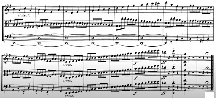
What happens when Meta’s aesthetic model encounters sustained rest in music? Not merely silence, but what Beethoven gives us in the final measures of his Opus 9 No 1: a quarter note followed by three beats of rest, then three more beats of rest, and finally an eighth note rest with a fermata. This isn’t an absence of sound, it is structured silence that creates meaning through anticipation and resolution. How can an algorithm chunking audio into 10-second segments possibly capture this temporal architecture of meaning?
Susanne K Langer, writing in Feeling and Form¹², that:
Musical duration is an image of what might be termed “lived” or “experienced” time-the passage of life that we feel as expectations become “now,” and “now” turns into unalterable fact. Such passage is measurable only in terms of sensibilities, tensions, and emotions; and it has not merely a different measure, but an altogether different structure from practical or scientific time.
The semblance of this vital, experiential time is the primary illusion of music. All music creates an order of virtual time, in which its sonorous forms move in relation to each other-always and only to each other, for nothing else exists there. Virtual time is as separate from the sequence of actual happenings as virtual space from actual space.
[...] music spreads out time for our direct and complete apprehension, by letting our hearing monopolize it-organize, fill, and shape it, all alone. It creates an image of time measured by the motion of forms that seem to give it substance, yet a substance that consists entirely of sound, so it is transitoriness itself. Music makes time audible, and its form and continuity sensible.
Music, then, is not merely organized sound that can be grasped outside its moment of articulation — it is the image of lived time itself.
Through music we express vital meanings that are simultaneously ontological and epistemological as music weaves the threads which give coherence to our experience of time, rescuing us from what is otherwise a metaphysically impoverished existence; one in which time is reduced to mere sequence, to clock-time’s endless succession of ideal events indifferent in themselves. This is precisely what Meta’s model, with its 10-second chunks and flattened metrics, fails to grasp: that musical meaning emerges not from the quantifiable features of sound, but from how music structures our very experience of temporality.
Langer’s insight into how music makes our internal lived time tangible highlights what has been at stake over the past 25 years of digital transformation in music production. With the rise of digital audio workstations, particularly Pro Tools, music-making underwent a fundamental shift: from existing primarily in an audial sphere to being mediated through visual waveforms and data points aligned to mechanical clock time. The consequences are profound — music became lines on a screen, measured against a grid representing ‘perfect’ timing, thereby annihilating the very lived time it was meant to express.
This griddification of music production reaches beyond method to fundamentally alter what music can ultimately express. When musical time is reduced to visual blocks on a timeline, When every note is quantized to perfect divisions of mechanical time, we lose something vital: the epistemological and ethical dimensions embedded in subtle temporal articulations, in the human variability that once conveyed lived experience beyond mere clock precision.
And yet(!) this flattening of musical time into grid-aligned data points was just the beginning. Through the mechanization of the music production process, these logics have laid the preconditions for something even more consequential: the emergence of these ‘aesthetic’ recommender systems. Meta’s aesthetic predictor model is not the first — by golly, I spent 17 years working on one myself, though with fundamentally different ontological assumptions and goals. These systems became possible precisely because musicians have already been conditioned to think of their work as quantifiable content, their artistic choices as optimizable variables. The temporal grid of Pro Tools paved the way for the reduction of aesthetic judgment to data points of potential ‘usefulness.’
Here we thought (musicians, especially session musicians) that all this technology was making us better, saving us invaluable time when mistakes happened under pressure — when the clock is ticking and 13 people are in the studio watching you do a take that is costing the label or songwriter $$$$$ an hour. ‘That backbeat you missed on the last measure of the bridge into the third verse? Don’t worry, we’ll just fly in a backbeat from another part of the song, it's all to the grid anyways.’
But what did those conveniences lead to? Those studios don’t exist anymore. We sit in our home studios, record our parts in isolation, sending stems back and forth digitally so we can lay a few takes down to the grid which will eventually end up as content on a Spotify playlist no one listens to intentionally or as a random stem analyzed by a team of 10 trained raters at Meta throwing that isolated drum track a 3 or maybe a 5 for Production Complexity depending on how many drum fills I get away with.
We’re all isolated content creators now, who are dependent on the machinic logics of platform capitalism to surface more content in the endless soup of mediocre nonsensical flattened aesthetics, which sort of fits a feeling I sort of had about something one time, which I am completely incapable of expressing anymore, and who cares anyways, no one has time to pay attention to it, intentionally.
Citations
¹ Tjandra, A., Wu, Y.-C., Guo, B., Hoffman, J., Ellis, B., Vyas, A., Shi, B., Chen, S., Le, M., Zacharov, N., Wood, C., Lee, A., & Hsu, W.-N. (2025). Meta Audiobox Aesthetics: Unified automatic quality assessment for speech, music, and sound. FAIR at Meta; Reality Labs at Meta. Retrieved from https://ai.meta.com/research/publications/meta-audiobox-aesthetics-unified-automatic-quality-assessment-for-speech-music-and-sound/
²A.W. Rix, J.G. Beerends, M.P. Hollier, and A.P. Hekstra. Perceptual evaluation of speech quality (pesq)-a new method for speech quality assessment of telephone networks and codecs. In IEEE International Conference on Acoustics, Speech and Signal Processing, ICASSP, 2001. doi: 10.1109/ICASSP.2001.941023.
³John G Beerends, Christian Schmidmer, Jens Berger, Matthias Obermann, Raphael Ullmann, Joachim Pomy, and Michael Keyhl. Perceptual objective listening quality assessment (polqa), the third generation itu-t standard for end-to-end speech quality measurement part i — temporal alignment. Journal of the Audio Engineering Society, 61 (6):366–384, 2013.
⁴ Tjandra, A., Wu, Y.-C., Guo, B., Hoffman, J., Ellis, B., Vyas, A., Shi, B., Chen, S., Le, M., Zacharov, N., Wood, C., Lee, A., & Hsu, W.-N. (2025). Meta Audiobox Aesthetics: Unified automatic quality assessment for speech, music, and sound. Retrieved from https://arxiv.org/abs/2502.05139
⁵ Wikipedia contributors. (n.d.). Music Genome Project. Wikipedia, The Free Encyclopedia. Retrieved from https://en.wikipedia.org/wiki/Music_Genome_Project
⁶ Sanyuan Chen, Chengyi Wang, Zhengyang Chen, Yu Wu, Shujie Liu, Zhuo Chen, Jinyu Li, Naoyuki Kanda, Takuya Yoshioka, Xiong Xiao, et al. Wavlm: Large-scale self-supervised pre-training for full stack speech processing. IEEE Journal of Selected Topics in Signal Processing, 16(6):1505–1518, 2022
⁷ Deshmukh, S., Alharthi, D., Elizalde, B., Gamper, H., Al Ismail, M., Singh, R., Raj, B., & Wang, H. (2024). PAM: Prompting audio-language models for audio quality assessment. arXiv. https://doi.org/10.48550/arXiv.2402.00282
⁸ Zafar Rafii, Antoine Liutkus, Fabian-Robert Stöter, Stylianos Ioannis Mimilakis, and Rachel Bittner. 2019. MUSDB18-HQ — an uncompressed version of MUSDB18. https://doi.org/10.5281/zenodo.3338373
⁹ MusicCaps. (2023). 5.5k high-quality music captions written by musicians. arXiv. https://doi.org/10.48550/arXiv.2301.11325
¹⁰ Jort F Gemmeke, Daniel PW Ellis, Dylan Freedman, Aren Jansen, Wade Lawrence, R Channing Moore, Manoj Plakal, and Marvin Ritter. Audio set: An ontology and human-labeled dataset for audio events. In 2017 IEEE international conference on acoustics, speech and signal processing (ICASSP), pages 776–780. IEEE, 2017.
¹¹ Anthony, J. (2025, January 11). No GPT-5 in 2025 and no AGI — Ever: The triadic nature of meaning-making and the fallacy of AI’s understanding. Medium. https://medium.com/@WeWillNotBeFlattened/no-gpt-5-in-2025-and-no-agi-ev
¹² Langer, S. K. K. (1953). Feeling and Form: A Theory of Art Developed from Philosophy in a New Key. United Kingdom: Routledge & Kegan Paul.